
Lung cancer is a leading global cause of cancer-related deaths. Detecting, predicting, and diagnosing it early is crucial for streamlined clinical management. In this project, I utilized machine learning (ML), specifically linear regression and random forest models, to identify high-risk individuals for lung cancer. Using a dataset of 535 individuals, I developed a web app allowing users to input symptoms and receive the likelihood of having lung cancer. The random forest model achieved high performance, with an AUC of 97% and R2 of 0.76, surpassing existing models in precision.
by R M Swin Ratnayake
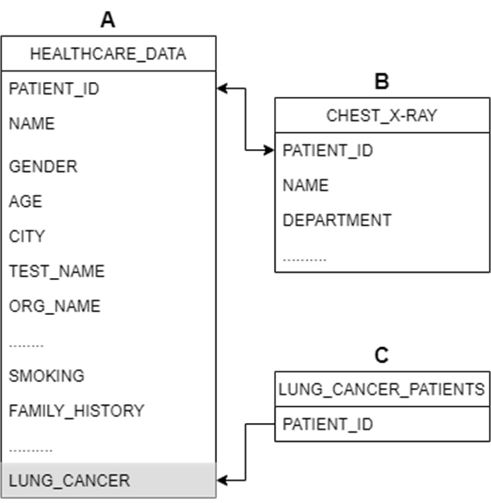
In this study, a comprehensive dataset was crucial, encompassing diverse features of lung cancer patients and those suspected of having lung cancer. To achieve this, data was sourced from the patient database of an oncology department, utilizing the CLIMS (Clinical Laboratory Information Management System). Despite the advanced capabilities of CLIMS, a single dataset with all relevant features proved elusive. Consequently, three distinct datasets were extracted and manipulated to craft the requisite data for this investigation.
To combine datasets A and B, the ‘PATIENT_ID’ entries were matched using the VLOOKUP feature in MS Excel. The formula used for this operation was:
=IF(ISNUMBER(VLOOKUP(Sheet1!A2,Sheet2!$A$2:$A$3937,1,FALSE)),Sheet1!A2,"")Afterward, the new dataset was filtered to exclude empty cells in the ID column, resulting in a refined dataset containing essential variables for suspected cancer patients.
To identify lung cancer patients, a new ‘LUNG_CANCER’ column was created using the VLOOKUP function to match IDs in Dataset A with those in Dataset C. The formula used for this purpose was:
=IF(ISNA(VLOOKUP(A2,Sheet3!$A$2:$A$372,1,FALSE)),"No","YES")In the realm of data analysis and machine learning, feature selection plays a pivotal role in determining the most crucial columns for a model’s accuracy. To refine our dataset, a meticulous process was employed. Initially, a manual filtering approach was implemented to eliminate non-essential factors, such as ‘SPEC_ITEMID,’ ‘SPEC_TYPE_DESC,’ ‘TEST_NAME,’ and others, as they were deemed redundant for the study’s objectives.
Subsequently, the feature ‘BLOOD_PRESSURE’ was excluded, considering no prior studies had established any correlation with lung cancer. For the remaining features, both a chi-squared test and Gini impurity analysis using Random Forest were conducted to assess their association with lung cancer.
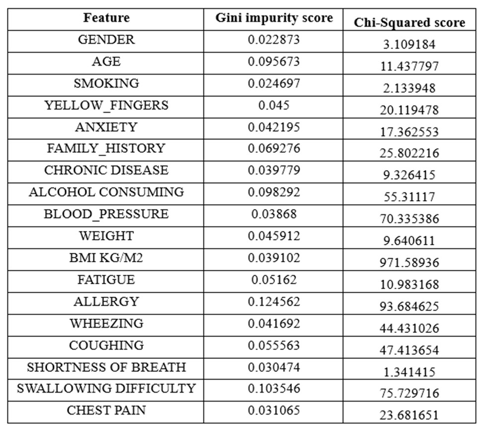
Chi-squared Test Feature Selection
The chi-squared test, employed to gauge significant correlations between two categorical variables, calculates a test statistic denoted as χ². This statistic reflects the discrepancy between observed (O) and expected (E) frequencies in a contingency table, with a higher χ² value indicating a stronger association between the variables.
Gini Impurity
Gini impurity, a measure of data impurity or randomness, was harnessed in conjunction with Random Forest for efficient feature selection. Defined as 1 - ∑(pi)^2, where pi represents the probability of each class in the dataset, Gini impurity ranges from 0 to 1. A score of 0 signifies a pure dataset, while 1 indicates a completely impure or random dataset.
The analysis, detailed in Table 1, led to the decision to remove the variable ‘BMI KG/M2’ due to its exceptionally high Chi-Squared score.
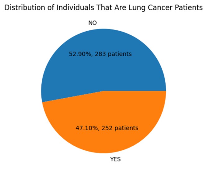
The final dataset after feature selection contains a total of 17 columns and 535 entries. 53% of the sample are cancer patients while 47% is healthy. Therefore, this dataset can be considered a balanced one as it is almost 1:1 ratio. This is an ideal scenario for many machine learning algorithms as it allows the model to learn equally from both classes and avoid any bias towards one class over the other.
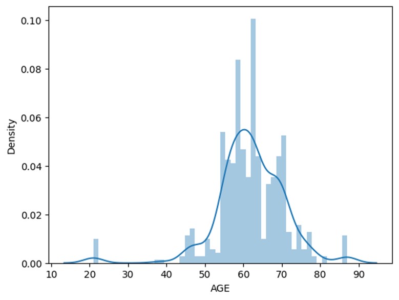
Histogram depicting the distribution of age in the sample population.
Most of the population sample is within the age range of 55 to 70. Age is an important risk indicator for the possibility of lung cancer. With age, its incidence rates rise, with those over 65 experiencing the greatest rates. The American Cancer Society (2022) reports that those aged 65 to 74 had the greatest incidence of lung cancer, followed by people 75 and older. In contrast, compared to those 65 to 74 years old, people 45 to 54 years old had a far lower risk of lung cancer. However, according to the heatmap age only has a co-relation of 0.12, this is a considerable low association.
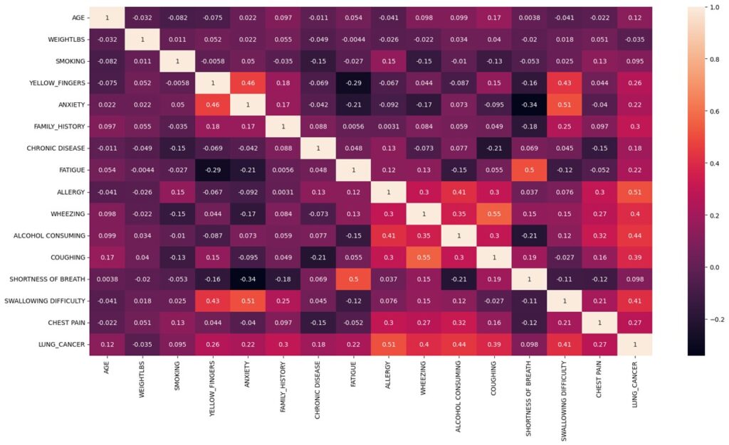
Heat map visual representation of the data’s distribution, patterns, and relationships.
A known risk factor for lung cancer is smoking. Nearly 80% of lung cancer fatalities, as per the American Cancer Society, are caused by smoking cigarettes. However, even though the heat map portrays that who did not smoke have less chance of having cancer it also shows evidence that those who smoke have an equal chance of having or not having cancer. There is a very low association between smoking and having lung cancer with a co-relation of 0.095. However, when we look at the bar graph for ‘YELLOW_FINGERS’ (a side-effect of heavy smoking) we can see that there is a direct co-relation between having yellow fingers and having lung cancer. Also, the heatmap shows that there is a correlation of 0.2. This could only mean that the dataset is flawed when it comes to determining smokers and non-smokers as patients are reluctant to mention the truth about their smoking habits with their doctor and that yellow fingers is a good metric to determine of the patient is a smoker.
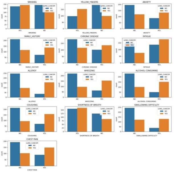
Bar graphs showing the number of individuals with and without lung cancer for each variable.
Every other feature shown in bar graphs above shows strong positive co-relation to having lung cancer except for individuals that have “SHOTRNESS OF BREATH”. Several studies have explored the relationship between shortness of breath and lung cancer and concluded that it is one of the most common symptoms of lung cancer. The graph shows that most people had shortness of breath, and this could be due to many other reasons, not necessarily lung cancer. Thus, visualizing the impression that shortness of breath has now affiliation to lung cancer.
The heat map shows that the variable with highest association to lung cancer is allergy with a co-relation of 0.51. Although some research has shown that those with allergies may have a decreased chance of getting lung cancer, other studies have found no conclusive evidence of a correlation, therefore the association between allergies and lung cancer is still not entirely understood. However, there is no medical evidence to prove a positive co-relation between allergy and lung cancer, as our data suggests. One possible explanation for this could be that both conditions share common risk factors, such as smoking or exposure to environmental pollutants. And another possibility is that the positive correlation is spurious and arises by chance. Alcohol consumption, swallowing difficulty and wheezing are other variables that show high positive co-relation as shown in heat map. There is a well-established link between these variables and lung cancer therefore we can conclude that the dataset has provided with true evidence for these variables. Weight on the other hand has a negative correlation of -0.035. This is because cancer patients tend to lose weight as a primary side effect.
To determine the most suited machine learning algorithm to develop the model, 2 different models were created, and the outcomes were evaluated. The 2 algorithms used to train the dataset are ‘Linear Regression’ and ‘Random Forest Regression’.
Random forest regression uses a group of decision trees to provide predictions. The data was separated into training and testing sets using the ‘train_test_split’ function. In our situation, 30% of the data is utilized for testing, while the remaining 70% is used for training. To guarantee that the split can be replicated, the random state of 42 is employed. The model is trained using the Random Forest technique once the data has been split. The model is created using the ‘RandomForestRegressor’ class of the ‘sklearn’ package. The Random Forest ensemble will utilize 100 decision trees, as specified by the ‘n_estimators’ option, which is set to 100. Then, using the training data as inputs, the model is subjected to the ‘fit’ procedure. This enables the model to learn the patterns in the data by training it on the training set.
Linear regression works by finding the coefficients of a linear equation that best fits the data points. The linear equation is of the form:
The first step in creating the model is to split the data into features and target variables. In our case, the ‘X’ variable contains all the features except for the target variable, ‘LUNG_CANCER’, while ‘y’ contains the target variable. The next step is to split the data into training and testing sets using the ‘train_test_split’ function. This is done to ensure that the model is trained on a subset of the data and tested on another subset to avoid overfitting. In our case, 20% of the data is used for testing, while 80% is used for training. The random state of 0 is used to ensure that the split is reproducible.
After the data is split, the model is trained using the Linear Regression algorithm. The ‘LinearRegression’ class of ‘sklearn’ package is used to create an instance of the model.
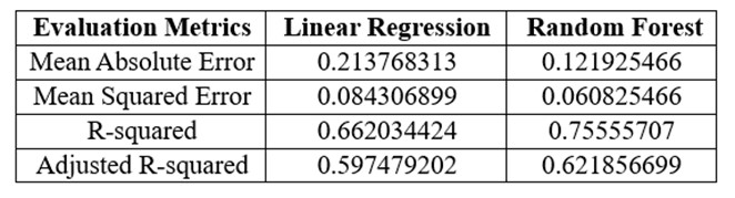
Results of each evaluation metric for machine learning models.
When it comes to choosing between the two algorithms, it is important to consider the performance of each model. Therefore, multiple evaluation techniques must be used to determine the best fitting model. In the evaluation metrics MAE and MSE, a lower value would mean a better performing model. As seen in table above, random forest regressor has a lower MAE and MSE when compared to linear regression model. When it comes to R2 and adjusted R2, the closer the value is to ‘1’, the better the performance of the model. As seen in table above, random forest regressor has a R2 and adjusted R2 value closer to ‘1’ when compared with linear regression. Therefore, all 4 of these metrics convey that random forest regressor is the best performing model for our dataset.
However, to further validate our choice, ROC curve plot and AUC value must be compared. AUC value is the area under the ROC curve plot ranging from 1 to 0. Therefore 0 indicates poor performance, and 1 indicates perfect performance.
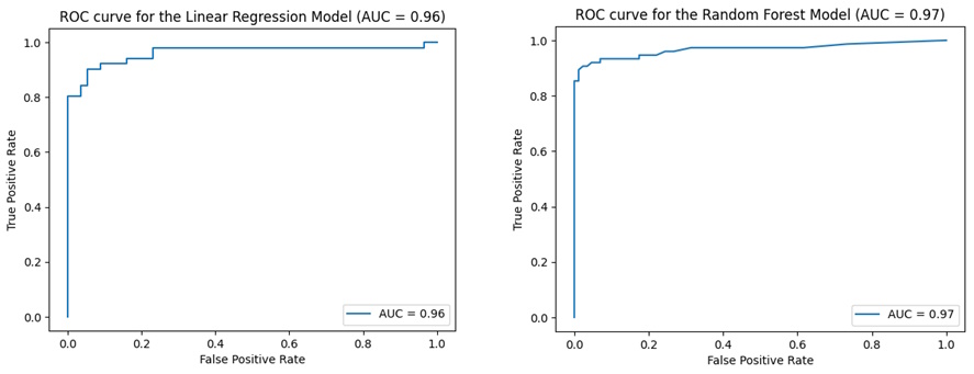
ROC curve plots and AUC values for each model
Linear regression model has an AUC value of 0.96 whereas, random forest has a value of 0.97. Both models have a score greater than 0.5 which means both have predictive ability. However, random forest has a higher value than linear regression which means random forest is a better-performing model, as it implies that the model can distinguish between positive and negative classes with high accuracy. Thus, further strengthening our choice to move forward with random forest regression to build the web app.
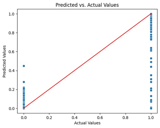
Predicted vs. actual values plot for random trees model.
The random tree model should be further analyzed in order to acquire a more thorough grasp of the model’s advantages and disadvantages and to make sure that the model is appropriate for the job at hand. A predicted vs. actual values plot was generated to gain insight into the model’s performance and identify areas for improvement. This method allows you to visually inspect the performance of the model and can help diagnose issues such as underfitting or overfitting. However, the plot shows the data point scattered in 2 horizontal line at ‘0’ and ‘1’ in the x-axis and not along the diagonal line. This doesn’t necessarily mean that the model has low performance. It is so because the actual values are binary and would therefore lie at ‘1’ and ‘0’. Therefore, a density contour plot must be generated with the datapoints to get a 3D aspect.
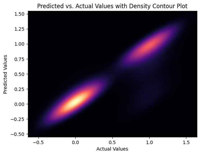
Predicted vs. actual values with density contour plot for the random tree model.
The predicted vs. actual values with density contour plot for the random tree model, unlike the predicted vs. actual plot this graph depicts the connection between the target variable’s actual values and anticipated values, along with a contour plot that shows the density of the data. Since the contours are close together and centered around the diagonal line this model can be considered a well-performing model. However, it too has clusters on the ‘0’ and ‘1’ points along the diagonal line. This is due to the nature of the dataset being binary values. However, this also means that these 2 points are the areas where the model is performing best.
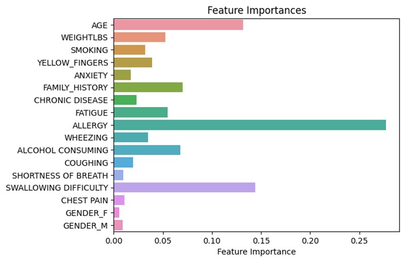
Feature plot portraying the importance of each feature on the outcome of the model.
The feature plot represents the importance of features in the random forest model on the result that will be shown in the web app. According to figure, ‘Allergy’ is the most important feature followed by ‘Swallowing Difficulty’ and ‘Age’. It also shows that ‘Shortness of Breath’ is the least important feature followed by ‘Chest Pain’ and ‘Gender’. However, this graph does not illustrate if the relevance is positive or negative.
Once I developed and evaluated the ML models, the most suitable model was exported using the ‘pickle’ library. Then ‘Flask’ was to create a web app that allows users to input their information and obtain a prediction of their lung cancer risk. The form and flask’s request object to obtain the user’s input was created using HTML. The user interface and result generation are shown below.
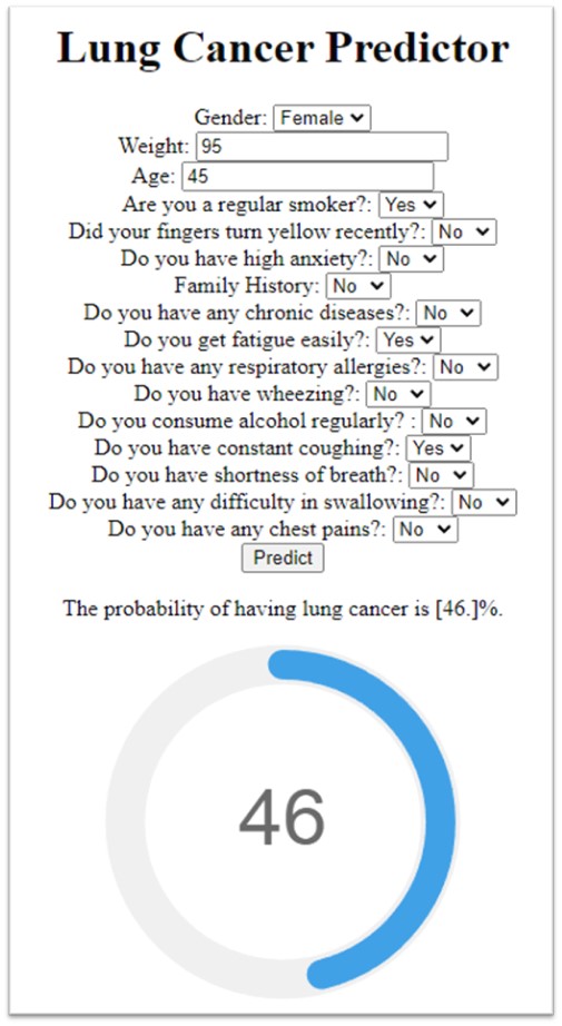
The user interface which gets user data and uses the ML model to generate the result.
In this project, I used supervised learning to create models that can identify people who have lung cancer indication based on a variety of traits and symptoms. The accuracy, precision, and AUC of 2 machine learning models, including linear regression and random forest regression, were assessed. Random forest regression beat linear regression according to the experiment findings and after applying multiple assessment metrics, with MAE, MSE, and R2 values of 0.12, 0.06, and 0.76, respectively, and an AUC of 97% (as seen in table 3) which is much greater than the performance we saw in most literatures. Therefore, it was used it to build the prognosis web app.
Future research will build on the current work by utilizing deep learning techniques, particularly artificial neural networks (ANN), long short-term memory (LSTM), and convolutional neural networks (CNN), to enrich the machine learning framework. The accuracy of the results will be compared to another research in the same field.
However, there are still considerable obstacles to the early identification of lung cancer even when this risk assessment tool is available. The poor adoption of lung cancer screening is one of the key obstacles, which may be ascribed to a number of things, including a lack of information among the general public and healthcare professionals, apprehension about radiation exposure, and worries about the expense of screening. Raising public and healthcare provider knowledge of the value of lung cancer screening and risk assessment is crucial for removing these obstacles. It’s critical to address the expense of lung cancer screening in addition to increasing awareness.
The creation of novel biomarkers and genetic testing techniques, as well as the use of cutting-edge technology like liquid biopsies, which examine a person’s blood for tumor DNA and other biomarkers, provide opportunities for improving early identification of lung cancer.